Acoustic cameras consist of microphone arrays used to locate and characterize sounds. There are a variety of microphone array structures to support specific analysis needs. Some acoustic cameras also have an embedded visual camera to supply an image over which the acoustic localization information can be presented. Acoustic camera application examples range from analyzing noise inside automobile cabins, aircraft, and trains, to quantifying the noise signature of wind turbines and monitoring industrial environments for anomalies and potential machine faults.
This FAQ begins with a brief overview of acoustic image algorithms including the application of artificial intelligence (AI), presents exemplary two- and three-dimensional microphone array structures, reviews how sound holography, localization, and monitoring work, and closes by looking at point-and-shoot acoustic cameras, sound scanners, and the simultaneous use of multiple microphone arrays.
An acoustic camera consists of a microphone array, a sound processing section, and a display. Microphone arrays can consist of dozens or hundreds of microphones. The sound processing section acquires the incoming sound information from the microphones simultaneously or with precise relative time delays. As the sound travels from the source, it arrives at the various microphones at different instances in time and with different intensities based on the relative locations of the microphones.
Beamforming is one method used for sound localization. It works by adding delays to the microphone signals and adding the signals to amplify the sound coming from a specific direction while minimizing or canceling the sound coming from other directions to essentially “point” the array in a specific direction. The calculated sound intensity information can be displayed on a power map.
Two techniques for sound localization are time difference of arrival (TDOA) and angle of arrival (AoA). They can be combined using a generalized cross-correlation (GCC) algorithm. GCC is relatively simple to implement and has low computational requirements. The tradeoff is that many microphones are needed to achieve accurate localization results. The use of a more complex algorithm can reduce the required number of microphones but will require a more capable (and more expensive) computational section with a faster processor and more memory.
Going beyond simple sound localization, sound intensity is quantified in dB and can be measured using acoustic probes. Some acoustic cameras include sound intensity and sound particle or pressure sensing measurement capabilities. Acoustic holography is another acoustical measurement technique and is used to determine the spatial propagation of acoustical waves or for the identification of acoustic sources. It is based on spatial Fourier transforms to estimate the near-field sound intensity around a source by using an array of particle velocity and/or pressure-sensing transducers.
Advanced acoustic cameras are available that combine digital microphones with AI. The use of AI-based measurement software enables developers to offer acoustic cameras with higher performance capabilities at a lower cost.
2D acoustic measurements
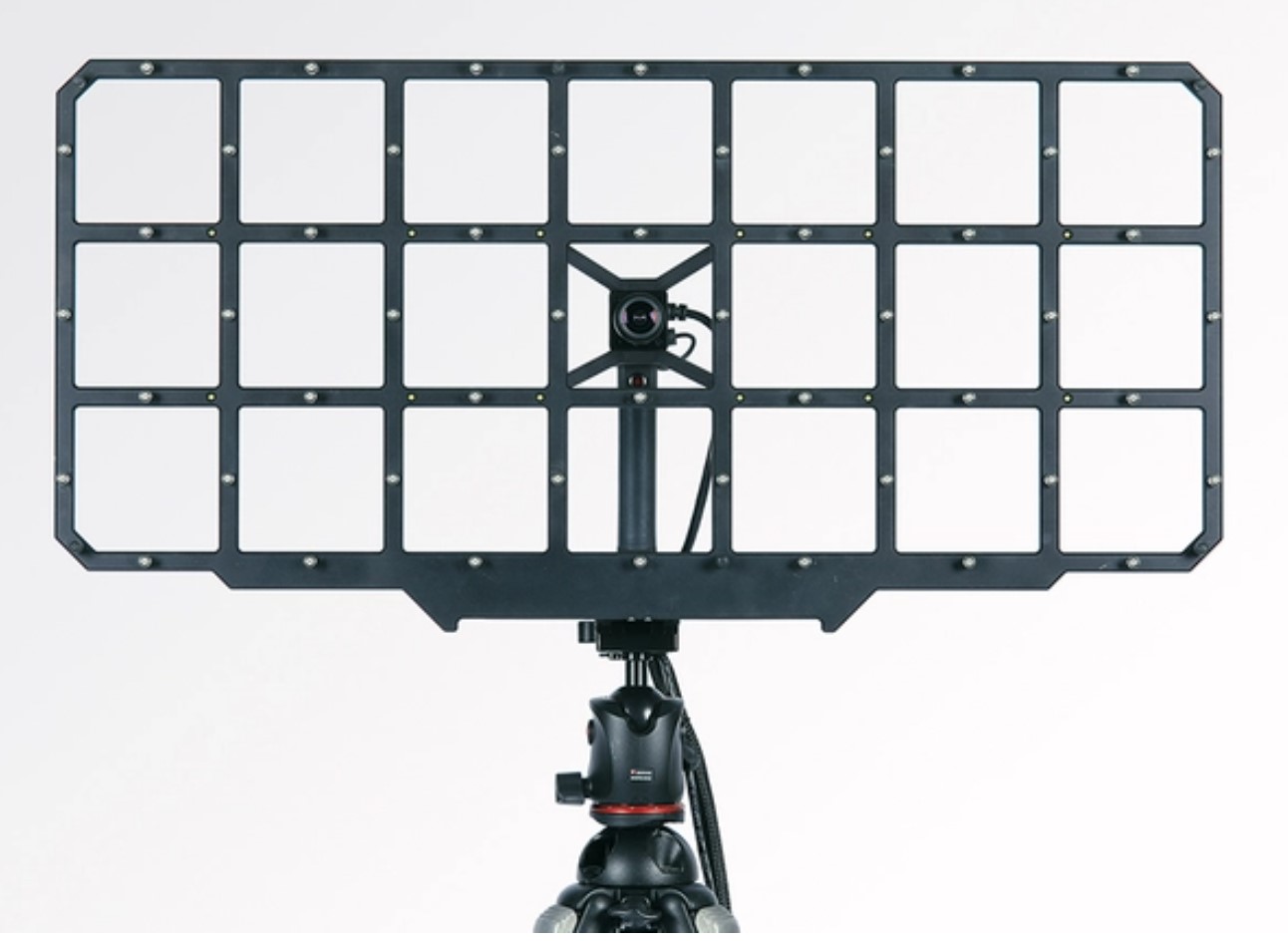
Two-dimensional (2D) acoustic mapping can be implemented using a variety of microphone array structures including rings, stars, octagons, Fibonacci structures, and rectangles, sometimes called paddles. The different structures provide varying performance options for near-field, far-field, and other mapping characteristics. These arrays all have unidirectional microphones all facing the same direction. 2D acoustic mapping is suited for measuring planar surfaces with the acoustic camera array perpendicular to the surface. Many surfaces are not completely flat making it difficult to produce precise measurements with a 2D array.
When 2D mapping is used to approximate three-dimensional (3D) surfaces into a plane, it can introduce measurement errors in the calculations of sound intensity. The approximations typically don’t account for the distance differences resulting from the surface being measured having different relative depths at different points. If the space is large, those errors can be small, but in small spaces, the error can be significant.
When implemented with a double-layer channel system of microphones, 2D arrays can implement near-field and far-field measurements using intensity mapping. In addition, with the necessary software, acoustic pressure can be mapped while particle velocity/acoustic intensity measurements are being mapped. Handheld 2D arrays are available for troubleshooting and portable applications while standalone arrays can provide higher precision laboratory and engineering-grade measurements. Various array structures are available that are suited for different applications:
- Ring arrays are suitable for beamforming and are used indoors and outdoors for far-field and near-field measurements.
- Star arrays are also suitable for beamforming and are mostly used for far-field measurements.
- Fibonacci arrays are suitable for holography or beamforming and can be used for near-field and far-field measurements with the same array. Based on a Fibonacci spiral pattern of the microphones, these arrays can provide a wider dynamic range compared to other structures.
- Paddle arrays are good low-frequency, near-field measurement tools (Figure 1).
3D acoustic measurements
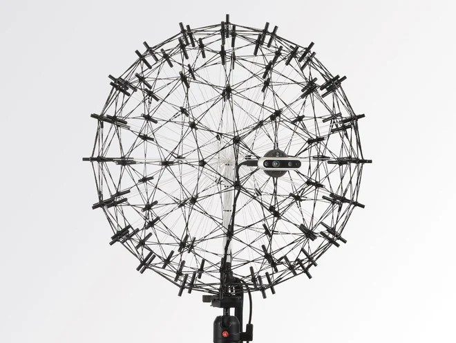
3D acoustic cameras consider surface nonlinearities and correct errors in measuring the distance between the microphone and the surface being measured. These cameras use a 3D model of the surface or space being analyzed. If the camera encounters a sound from a source that is not included in the model, errors can arise like mapping the sound to a random location, or the sound may be eliminated from the measurements.
3D acoustic cameras are especially suited for analyzing enclosed spaces like room or vehicle interiors. These cameras consist of a sphere of microphones, with each microphone pointing outward perpendicularly to the surface of the sphere, that can provide omnidirectional sound measurements (Figure 2). These cameras often employ beamforming with the measurements mapped into 3D point clouds or a 3D computer-aided drawing (CAD) model of the environment being measured.
Point-and-shoot acoustic imagers
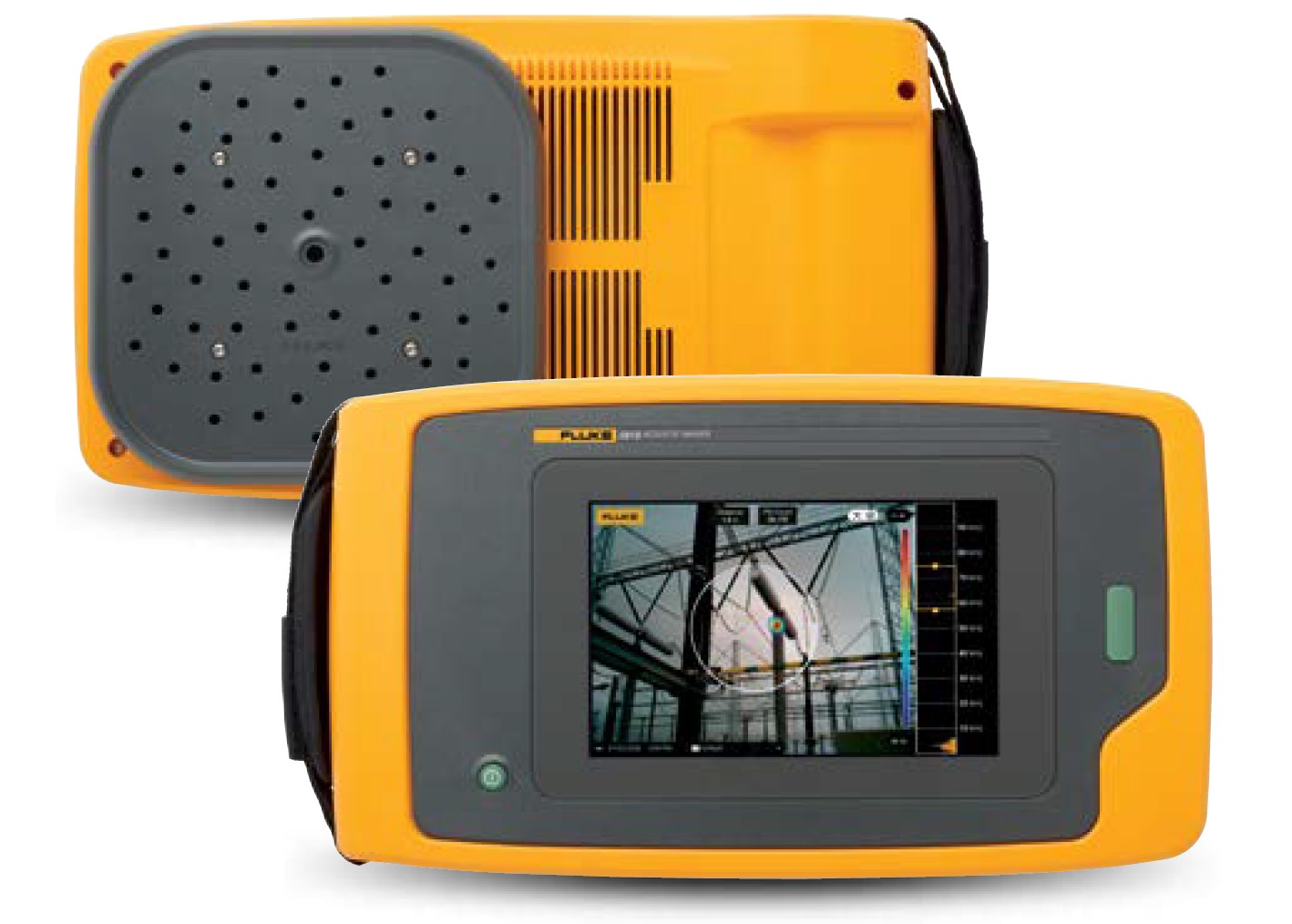
A handheld acoustic imager has been developed for applications like identifying leaks in compressed air, gas, steam, and vacuum systems and detecting and localizing partial discharge conditions in insulators, transformers, switch gears, or high voltage (HV) powerlines. The 64 microphones in the acoustic array operate from 2 to 100 kHz with a detection range of up to 120 meters. The array has a field of view of 63° ± 5° and takes images at a rate of 25 frames per second. The integrated digital camera has the same field of view plus a 3x digital zoom capability with a resolution of 5 megapixels. In addition to displaying still images, the system can take videos up to 5 minutes long (Figure 3). To minimize background noise interference, the imager automatically compensates for background noise and has multiple bandwidths that are selectable via manual inputs or with user-made presets.
Sound scanners
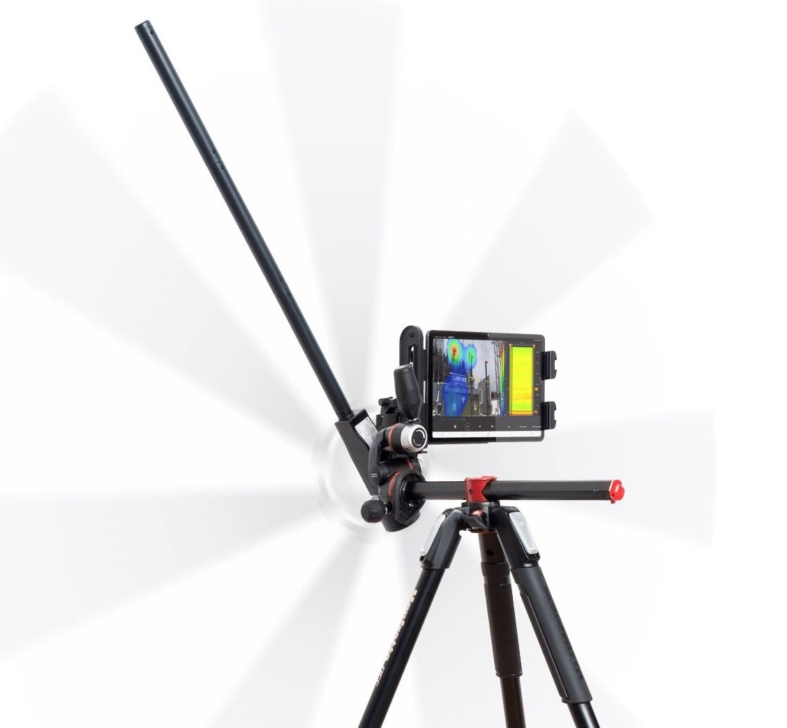
Devices called sound scanners are available that can simulate up to 480 microphone positions using 5 microphones on a boom that’s rotated in a circle (Figure 4). The scanner has been developed specifically for use in field measurements since it’s lightweight and compact making it easy to transport. It’s intended for use in building acoustics and environmental noise measurements. The 1.32-meter diameter of the sensor structure means that precision visualization of low-frequency sounds is supported.
The scanner system is self-contained and battery-powered and does not require a laptop computer, external data recorder, or power adapter. The system includes five components:
- Rotating sensor unit
- Mobile electronics
- Software
- Supporting cloud infrastructure
- Tripod
Two arrays can be better than one
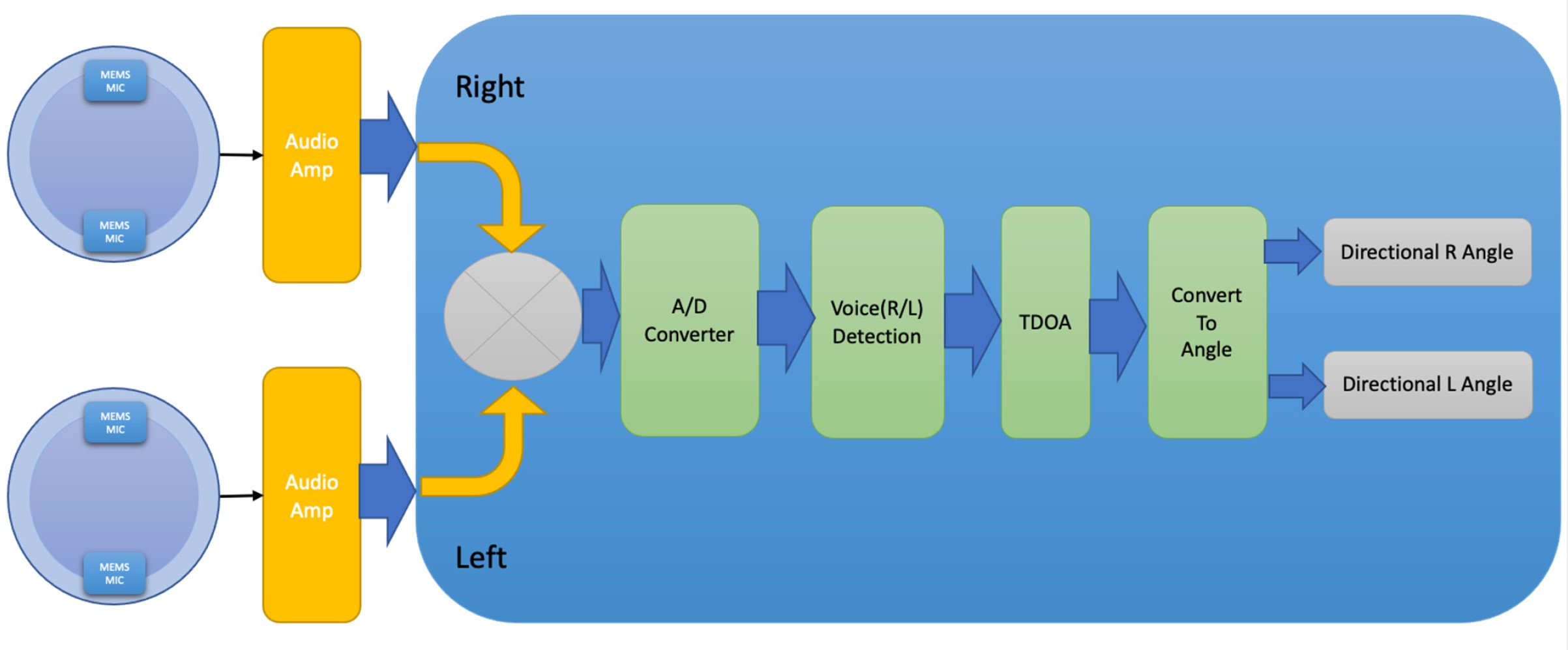
A new method has been proposed that uses two microphone arrays with only two microphones in each array to form ‘left’ and ‘right’ channels. TDOA was used to convert the channels into angles, using simple GCC without additional algorithms (Figure 5). A prototype of this two-channel approach produced a position error of about 2.3 cm and an angle error of about 0.74 degrees using only four microphones in an indoor environment.
Summary
Acoustic cameras are a well-established technology and include both 2D and 3D imaging systems. They use algorithms based on techniques like beamforming, sound intensity measurements, and acoustic holography. The addition of AI is enabling the development of high-performance acoustic cameras at a lower cost. In addition, techniques are being developed that enable fewer microphones to be used to produce high-accuracy measurements, further reducing the cost of employing acoustic cameras.
References
Acoustic Camera, Wikipedia
An Acoustic Camera for Use on UAVs, MDPI sensors
Microphone Arrays for Different Applications, gfai tech
Precision Acoustic Imager, Fluke
Sound Localization Based on Acoustic Source Using Multiple Microphone Array in an Indoor Environment, MDPI electronics
Sound Scanner, Seven Bel